Usage¶

Recommendation¶

The ORIGIN algorithm is computationally intensive, hence it is divided in steps. It is possible to save the outputs after each step and to reload a session to continue the processing.

The software has been originally developed for the MUSE Hubble Ultra-Deep Field (Bacon et al, 2017). Although it was extensively tested on these deep datacubes, the blind use of the software is not recommended and the user is advice to run each step, check carefully the results and play with the input parameters until satisfactory results are obtained.

The quality of the input cube is key to obtain the maximum detections and to limit the false detections. The algorithm is able to learn from the datacube itself its noise properties and to adapt the threshold and other parameters. However it has not been tested with strong non-gaussian noise or large systematics.

The ORIGIN class¶

To run ORIGIN everything can be done through the ORIGIN object. To instantiate this object, we need to pass it a MUSE datacube. Here for the example we will use the MUSE cube stored in the muse_origin package, which is also used for the unit tests:

>>> import muse_origin
>>> import os
>>> origdir = os.path.dirname(muse_origin.__file__)
>>> CUBE = os.path.join(origdir, '..', 'tests', 'minicube.fits')

This supposes that you use a full copy of the git repository, the tests are not included in the Python package because the file is quite big.

We also must give it a name, this is the “session” name which is used as the directory name in which outputs will be saved (inside the current directory by default, which can be overridden with the path argument):

>>> testpath = getfixture('tmpdir')
>>> orig = muse_origin.ORIGIN(CUBE, name='origtest', loglevel='INFO', path=testpath)
INFO : Step 00 - Initialization (ORIGIN ...)
INFO : Read the Data Cube ...
INFO : Compute FSFs from the datacube FITS header keywords
INFO : mean FWHM of the FSFs = 3.32 pixels
INFO : 00 Done

Then this object allows to run the steps, which is described in more details in the example notebook. It is possible to know the status of the processing with status:

>>> orig.status()
- 01, preprocessing: NOTRUN
- 02, areas: NOTRUN
- 03, compute_PCA_threshold: NOTRUN
- 04, compute_greedy_PCA: NOTRUN
- 05, compute_TGLR: NOTRUN
- 06, compute_purity_threshold: NOTRUN
- 07, detection: NOTRUN
- 08, compute_spectra: NOTRUN
- 09, clean_results: NOTRUN
- 10, create_masks: NOTRUN
- 11, save_sources: NOTRUN

Inputs¶

Datacube¶

The input datacube must follow the MUSE standards, with proper WCS information and data and variance extensions.

When the SNR is too low at the edge of the field, it might be wise to mask these regions or to truncate the datacube. These operations can be easily done in MPDAF with the Cube Class.

FSF¶

ORIGIN needs some information about the FSF (Field Spread Function), including its dependency on the wavelength. The FSF model can be read from the cube with MPDAF’s FSF models (mpdaf.MUSE.FSFModel) or it can be provided as parameter. It is also possible to use a Fieldmap for the case of mosaics where the FSF varies on the field.

By default ORIGIN supposes that the cube contains an FSF model that can be read with MPDAF:

>>> from mpdaf.MUSE import FSFModel
>>> fsfmodel = FSFModel.read(CUBE)
>>> fsfmodel
<MoffatModel2(model=2)>
>>> fsfmodel.to_header().cards
('FSFMODE', 2, 'Circular MOFFAT beta=poly(lbda) fwhm=poly(lbda)')
('FSFLB1', 5000, 'FSF Blue Ref Wave (A)')
('FSFLB2', 9000, 'FSF Red Ref Wave (A)')
('FSF00FNC', 2, 'FSF00 FWHM Poly Ncoef')
('FSF00F00', -0.136046443480448, 'FSF00 FWHM Poly C00')
('FSF00F01', 0.6312330752702884, 'FSF00 FWHM Poly C01')
('FSF00BNC', 1, 'FSF00 BETA Poly Ncoef')
('FSF00B00', 2.8, 'FSF00 BETA Poly C00')

This model is used to get the FWHM for each wavelength plane, otherwise the full list must be provides as parameter:

>>> import numpy as np
>>> fsfmodel.get_fwhm(np.array([5000, 7000, 9000]))
array([0.69... , 0.63..., 0.56...])

Note

Although ORIGIN would perform better with an accurate FSF model, it is not very sensitive to its exact shape. It is recommended to derive a FSF model with MPDAF’s FSF models and to save it in the datacube.

Profiles¶

For the spectral axis ORIGIN uses a dictionary of line profiles, which will be used to compute the spectral correlation. The ORIGIN comes with two FITS files containing profiles:

Dico_3FWHM.fits: contains 3 profiles with FWHM of 2, 6.7 and 12 pixels. This is the one used by default.
Dico_FWHM_2_12.fits: contains 20 profiles with FWHM between 2 and 12 pixels.

Note

The CPU time for the TGLR computation ComputeTGLR is directly proportional to the number of profiles.

Session save and restore¶

At any point it is possible to save the current state with write:

>>> orig.write()
INFO : Writing...
INFO : Current session saved in .../origtest

This uses the name of the object as output directory:

>>> orig.name
'origtest'

In this output directory, all the step outputs are saved, as well as a log file ({name}.log) and a YAML file with all the parameters used in the various steps ({name}.yaml).

A session can then be reloaded with load:

>>> import muse_origin
>>> orig = muse_origin.ORIGIN.load(os.path.join(testpath, 'origtest'))
INFO : Step 00 - Initialization (ORIGIN ...)
INFO : Read the Data Cube ...
INFO : Compute FSFs from the datacube FITS header keywords
INFO : mean FWHM of the FSFs = 3.32 pixels
INFO : 00 Done

Another interesting point with the session feature is that saving the current state will unload the data from the memory. When running the steps, various data objects (cubes, images, tables) are added as attributes to the step classes, and saving the session will dump these objects to disk and free the memory.

Steps¶

The steps are implemented are Step sub-classes (described below), which can be run with methods of the ORIGIN object:

orig.step01_preprocessing
orig.step02_areas
orig.step03_compute_PCA_threshold
orig.step04_compute_greedy_PCA
orig.step05_compute_TGLR
orig.step06_compute_purity_threshold
orig.step07_detection
orig.step08_compute_spectra
orig.step09_clean_results
orig.step10_create_masks
orig.step11_save_sources

Each step has several parameters, with default values. The most important parameters are mentioned below, and more details about the others parameters and attributes can be found in the docstrings of the step classes.

Step 1: Preprocessing

Preparation of the data for the following steps:

Nuisance removal with DCT. The estimated continuum cube is stored in cube_dct. The order of the DCT is set with the dct_order keyword.
Standardization of the data (stored in cube_std).
Computation of the local maxima and minima of cube_std.
Segmentation based on the continuum (segmap_cont), with the threshold defined by pfasegcont.
Segmentation based on the residual image (ima_std), with the threshold defined by pfasegres, merged with the previous one which gives segmap_merged.

Step 2: CreateAreas

Creation of areas for the PCA.

The purpose of spatial segmentation is to locate regions where the sky contains “nuisance” sources, i.e., sources with continuum and / or bright emission lines, or regions exhibiting a particular statistical behaviour, caused by the presence of systematic residuals for instance.

The merged segmentation map computed previously is used to avoid cutting continuum objects. The size of the areas is controlled with the minsize and maxsize keywords.

Step 3: ComputePCAThreshold

Loop on each area and estimate the threshold for the PCA, using the pfa_test parameter.

This parameter is important. If it is too small, the PCA will not be efficient to remove the background residuals and the algorithm will fail to detect faint emitters. It if is too important, the risk is to remove the line emitters. Note that the algorithm is able to retrieve the brightest line emitters which have been removed by the PCA.

Step 4: ComputeGreedyPCA

Nuisance removal with iterative PCA.

This is one of the most computationally intensive step in ORIGIN, with the following step.

Loop on each area and compute the iterative PCA: iteratively locate and remove residual nuisance sources, i.e., any signal that is not the signature of a faint, spatially unresolved emission line. Use by default the thresholds computed in step 3.

Inspection of the map of the number of PCA iterations is instructive of the regions of low SNR and/or defects in the datacube. Depending of the datacube quality, the default value of the maximum number of iterations might be increase.

Step 5: ComputeTGLR

Compute the cube of GLR test values (the “correlation” cube).

The test is done on the cube containing the faint signal (cube_faint) and it uses the PSF and the spectral profiles. Then computes the local maximum and minima of correlation values and stores the maxmap and minmap images. It is possible to use multiprocessing to parallelize the work (with n_jobs), but the best is to use the c-level parallelization with the mkl-fft package.

Warning

Do not use both n_jobs and mkl-fft, this will result in too many threads and will slow down the computation.

Step 6: ComputePurityThreshold

Find the thresholds for the given purity, for the correlation (faint) cube and the complementary (std) one.

Tip

The purity computation can fail if the number of detections in the negative cube is always larger than in the positive datacube. If this happen, it is still psossible to continue to next step by fixing the threshold parameter. Inspection of the purity plot can help to find the correct threshold to avoid too many false detections.

Step 7: Detection

Detections on local maxima from the correlation and complementary cube, using the thresholds computed in step 5. It is also possible to provides thresholds with the corresponding parameters. This creates the Cat0 table.

Then the detections are merged in sources, to create Cat1. See Merging of lines in sources below.

Step 8: ComputeSpectra

Compute the estimated emission line and the optimal coordinates.

This computes Cat2 with a refined position for sources. And for each detected line in a spatio-spectral grid, the line is estimated with the deconvolution model:

subcube = FSF*line -> line_est = subcube*fsf/(fsf^2))

Warning

The line flux value reported in the Cat2 table is buggy. To get correct flux value, it is recommended to extract them from the spectrum stored in the final source computation step.

Step 9: CleanResults

This step does several things to “clean” the results of ORIGIN:

Some lines are associated to the same source but are very near considering their z positions. The lines are all marked as merged in the brightest line of the group (but are kept in the line table).
A table of unique sources is created.
Statistical detection info is added on the 2 resulting catalogs.

This step produces two tables:

Cat3_lines: clean table of lines;
Cat3_sources: table of unique sources.

Step 10: CreateMasks

This step create a source mask and a sky mask for each source. These masks are computed as the combination of masks on the narrow band images of each line.

Step 11: SaveSources

Create an mpdaf.sdetect.Source file for each source. See Source content for detailed information of the source content.

Merging of lines in sources¶

Once we get the list of line detections, we need to group these detections in “sources”, where a given source can have multiple lines. It’s a tricky step because extended sources can have detections with different spatial positions. To solve this problem we use the information from a segmentation map, that can be provided or computed automatically on the continuum image, to identify the regions of bright or extended sources. And we adopt a different method for detections that are in these areas.

First, the detections are merged based on a spatial distance criteria (the tol_spat parameter). Starting from a given detection, the detections within a distance of tol_spat are merged. Then looking iteratively at the neighbors of the merged detections, these are merged in the group if their distance to the seed detection is less than tol_spat, or if the distance on the wavelength axis is less than tol_spec. And this process is repeated for all detections that are not yet merged.

Then we take all the detections that belong to a given region of the segmentation map, and if there is more than one group of lines from the previous step we compute the distance on the wavelength axis between the groups of lines. If the minimum distance in wavelength is less than tol_spec then the groups are merged.

Source content¶

For each detected source a FITS file is created. This file can be inspected using the MPDAF mpdaf.sdetect.Source package. It contains informations stored in its header and a list of images, tables, cubes and spectra.

Example:

>>> from mpdaf.sdetect.source import Source
>>> src = Source.from_file('orig_mxdf/sources/source-00046.fits')  
>>> src.info()  
[INFO] ID      =                   46 / object ID %d
[INFO] RA      =    53.16711704003818 / RA u.degree %.7f
[INFO] DEC     =   -27.79575893776533 / DEC u.degree %.7f
[INFO] FROM    = 'ORIGIN  '           / detection software
...
[INFO] OR_NG   =                    3 / OR input, connectivity size
[INFO] OR_DXY  =                    3 / OR input, spatial tolerance for merging (pix)
[INFO] OR_DZ   =                    5 / OR input, spectral tolerance for merging (pix)
[INFO] OR_NXZ  =                    0 / OR input, grid Nxy
[INFO] COMP_CAT=                    0 / 1/0 (1=Pre-detected in STD, 0=detected in CORRE
[INFO] OR_TH   =                 6.92 / OR input, threshold
[INFO] OR_PURI =                  0.8 / OR input, purity
[INFO] REFSPEC = 'ORI_CORR_230_SKYSUB'
[INFO] FORMAT  = '0.6     '           / Version of the Source format
[INFO] HISTORY [0.0] Source created with ORIGIN (RB 2020-01-17)
[INFO] 9 spectra: MUSE_SKY MUSE_TOT_SKYSUB MUSE_WHITE_SKYSUB MUSE_TOT MUSE_WHITE ORI_CORR ORI_SPEC_230 ORI_CORR_230_SKYSUB ORI_CORR_230
[INFO] 9 images: MUSE_WHITE ORI_MAXMAP ORI_MASK_OBJ ORI_MASK_SKY ORI_SEGMAP_LABEL ORI_SEGMAP_MERGED EXPMAP NB_LINE_230 ORI_CORR_230
[INFO] 2 cubes: MUSE_CUBE ORI_CORREL
[INFO] 3 tables: ORI_CAT ORI_LINES NB_PAR
[INFO] 1 lines

The table ORI_LINES contain line information:

>>> src.tables['ORI_LINES']  
    <Table masked=True length=1>
ID          ra                dec            lbda     x   ... line_merged_flag merged_in      nsigTGLR      nsigSTD
int64      float64            float64       float64 int64 ...       bool         int64        float64       float64
----- ----------------- ------------------- ------- ----- ... ---------------- --------- ------------------ -------
142 53.16010113941778   -27.786101772517704  5772.5   178 ...            False        -- 29.074403824269364     nan

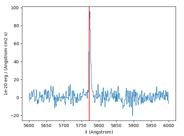
The source spectrum is also available:

>>> import matplotlib.pyplot as plt
>>> fig = plt.figure()  
>>> src.spectra[src.REFSPEC].plot(lmin=5600,lmax=6000)  
>>> plt.axvline(5772.5, color='r')  
>>> plt.show()  

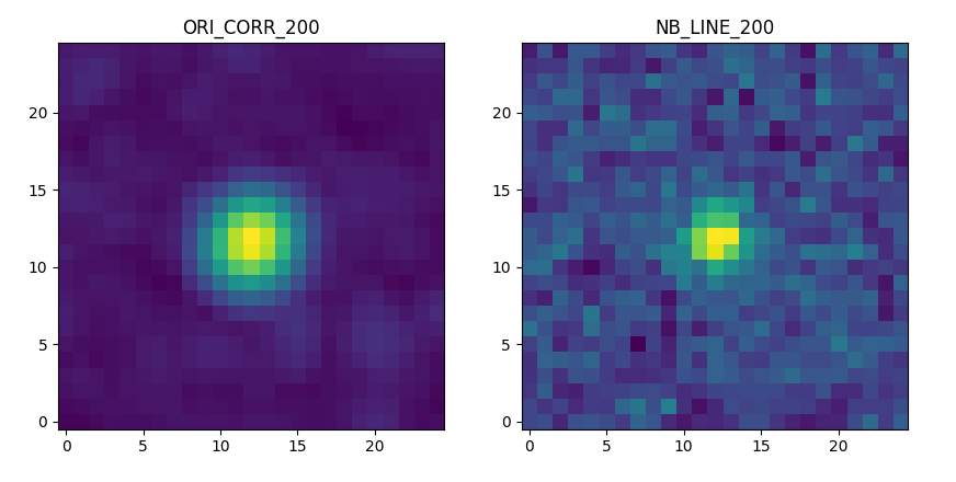
and the correlation and narrow band images:

>>> fig,ax = plt.subplots(1,2,figsize=(10,5))  
>>> src.images['ORI_CORR_200'].plot(ax=ax[0], title='ORI_CORR_200')  
>>> src.images['NB_LINE_200'].plot(ax=ax[1], title='NB_LINE_200')  
>>> plt.show()  